Two of our esteemed OPIGlets presented a workshop on collaborative research using Jupyter Notebook this week at ISMB in Chicago. Their workshop highlights the importance of finding ways to share your work conveniently and reproducibly. So on a related note, I thought I would share a brief introduction to another useful tool, R Markdown with RStudio, which I use to present updates to various supervisors and to remember what I did three months (or three days) ago. This method of sharing work is highly readable, reproducible, and narrative-driven.
I use R for much of my data analysis and all of my visualisation, and I count the tidyverse among my most beloved friends. If you’re so inclined, it’s easy to execute python, bash, and more from within R Markdown. You also don’t need to use RStudio to use R Markdown, but that’s a whole other story.
Starting a new markdown file in RStudio will generate a template script explaining most of what you need to know. If I showed you that then I’d be out of a blog post, but I will at least link to the R Markdown Reference Guide.
R Markdown files consist of text written in markdown, and code chunks that can be individually executed and displayed inline within RStudio. To “knit” the whole thing together, the knitr package is used to execute and combine code chunks, then pandoc converts the whole thing into an attractive document.
Here’s an example. The metadata at the top sets up the document. I’ll be generating an html document here, but notice some other tempting examples commented out. Yes, you can use it for Latex (swoon). You can even make a Word document, but really, why would you?
---
title: "Informative Title"
author: "Clare E. West"
date: "10/07/2018"
output: html_document
#output: beamer_presentation
#output: pdf_document
---
```{r setup, include=FALSE}
knitr::opts_chunk$set(echo = TRUE)
library(knitr)
library(ggplot2)
library(tidyr)
library(dplyr)
```
## Big Title
### Smaller title
R Markdown scripts have the extension .Rmd
R Markdown is __so__ *fun*. You can read all about it [here](https://www.rstudio.com/wp-content/uploads/2015/03/rmarkdown-reference.pdf).
```{r}
print("Hello world")
```
Notice that chunks are enclosed within three backticks, with the language and options in braces. Single commands can be executed inline using single backticks.
As highlighted in the example above, global options are set like this:
knitr::opts_chunk$set(echo = TRUE)
echo=TRUE means that the code in each chunk is displayed in the final product; this is useful to show collaborators (or your future self) exactly how you did something. Change this option (echo = FALSE) globally or in individual blocks to prevent code from printing. This is useful to hide uninteresting commands, or when presenting to people who don’t have the time or inclination to read your code (hard to imagine). Notice I’ve also used include = FALSE for the library-loading code chunk, which means evaluate but don’t include in the output. Another useful option is eval = FALSE, which means don’t even run this chunk.
So let’s see what that looks like when we render it:
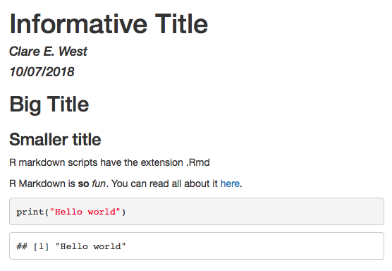
The above example output as HTML
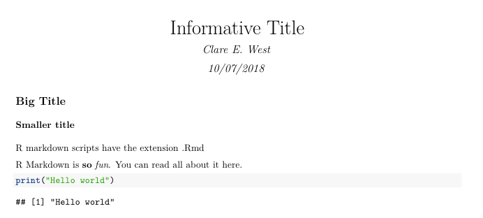
The above example output as Latex
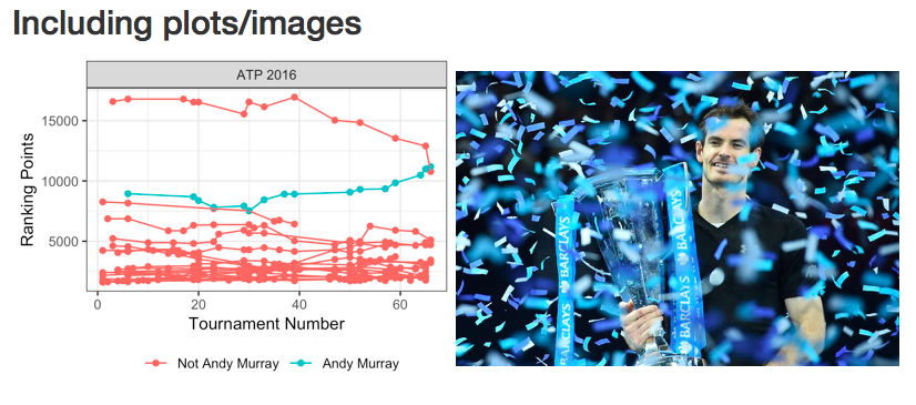
Plots generated in code chunks or images from other sources can be embedded. Set the width in the options. “fig.width” sets the width (in inches) of the figure generated, while “out.width” scales the image in the final documents, for which the units will depend on the document type. Within RStudio, these are previewed inline below the code chunk.
## Including plots/images
```{r fig.width = 4, fig.height = 3, out.width = "400px", echo=FALSE}
t  %>% group_by(Tour, Winner, N, Tournament) %>% filter(WRank <= 20) %>% summarise(WPts = max(WPts))  %>% ggplot(aes(x=N, y=WPts, group=Winner, colour=(Winner=="Murray A."))) + geom_point() + geom_line() + labs(x="Tournament Number",y="Ranking Points") + scale_colour_discrete("",labels=c("Not Andy Murray", "Andy Murray")) + theme_bw() + theme(legend.position = "bottom", legend.margin = margin(0, 0, 0, 0))
knitr::include_graphics("https://s.yimg.com/ny/api/res/1.2/69ZUzNSMYb09GKd8CNJeew--~A/YXBwaWQ9aGlnaGxhbmRlcjtzbT0xO3c9ODAwO2g9NjAw/http://media.zenfs.com/en_us/News/afp.com/0102e1f7d0d3c35303c8a62d56a5eb79c2c8b4d8.jpg")
```
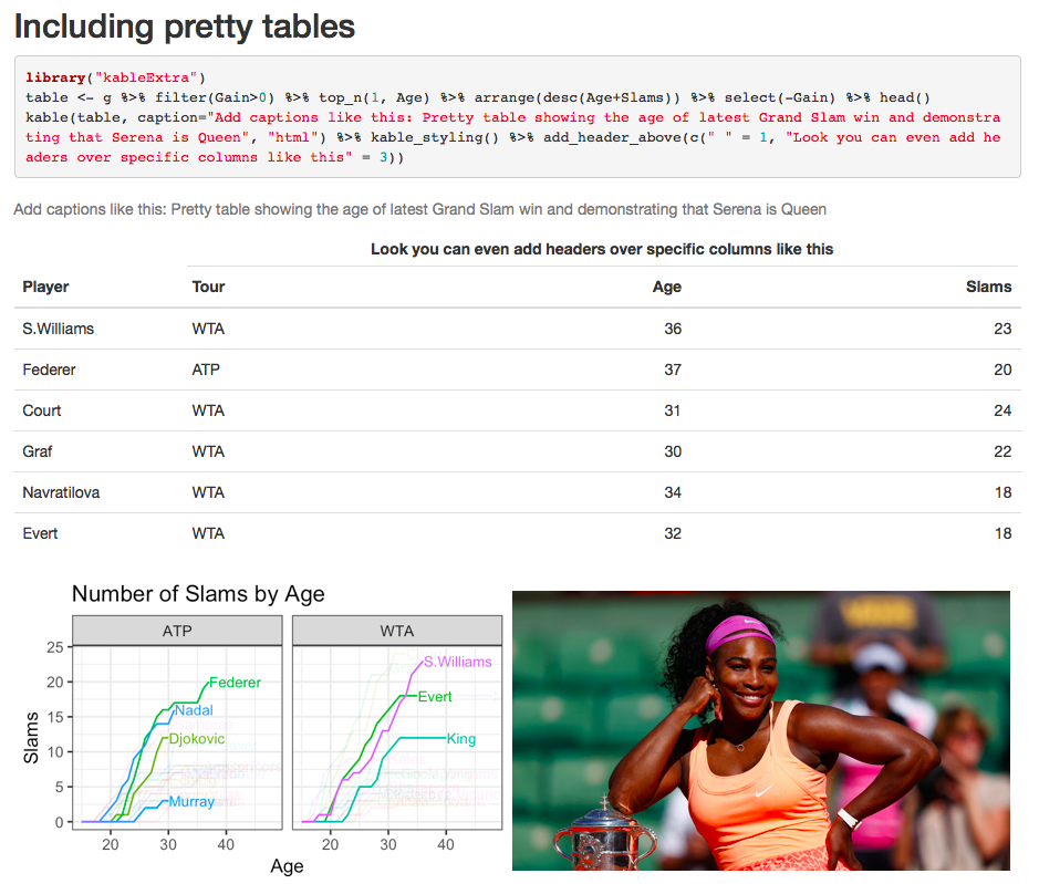
Rather than just printing data R-style, you can nicely format it into a table using kable (part of knitr). I also style mine using kableExtra, which makes it look nice and gives you extra options. By default tables fill the full width, you can override this using e.g. kable_styling(full.width = FALSE, position = “left”). When making a latex document, use kable(table, booktabs = T, “latex”) to get a (reproducible) latex-style table.
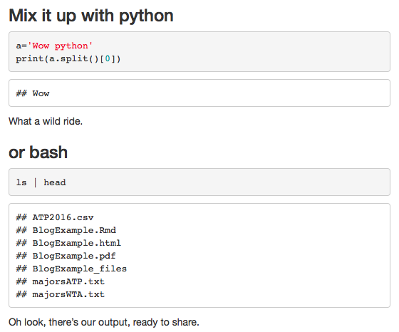
Here’s how to use python and bash. Thanks to the package reticulate, you can even share objects between your R and Python chunks. Exclude reticulate with knitr::opts_chunk$set(python.reticulate=FALSE) if you prefer to keep your languages separate.
### Mix it up with python
```{python}
a='Wow python'
print(a.split()[0])
```
What a wild ride.
### or bash
```{bash, echo=TRUE}
ls | head
```
Oh look, there's our output, ready to share.
Finally, if you hate GUIs – and you know I do – you can ditch the interactive notebook part and just generate documents from R Markdown files like this:
rmarkdown::render("BlogExample.Rmd")
This blog post was originally posted on the OPIG blog.